For_Loops
Noah W.K. Mattheis
2025-02-25
Going over Loops/For Loops/ While Loops
For Loops can be slow in R, especially when using functions like cbind in a loop R is a language that doesn’t need to rely on them too much So why do we use them? Comfort, ease of transfer to other languages, sometimes easier to read, and sometimes laziness
BASIC ANATOMY OF FOR LOOP
for (var in seq) { start of for loop
body of for loop
} end of for loop
Good rule of thumb - Use i, j, or k for the var of loop This way, we know if we are using these counter variables, we know we are in a loop Common etiquette across other languages as well, like Java and Python
General way to set up for loops
for (i in 1:5) { # initializes loop and will iterate 5 times
  cat("stuck in a loop", "\n") # First will print/concatenate this line
  cat(3 + 2, "\n") # then will do this arithmetic
  cat(runif(1), "\n") # then will create a rand unif number
} # Loop will run 5 times, as we specified, before it is finished
## stuck in a loop
## 5
## 0.5028801
## stuck in a loop
## 5
## 0.6269116
## stuck in a loop
## 5
## 0.1350145
## stuck in a loop
## 5
## 0.6696389
## stuck in a loop
## 5
## 0.5565729For loops can also iniate/reassign values
## [1] 1
## [1] 3
## [1] 6
## [1] 10
## [1] 15
For loop with iterations based on vector length
my_dogs <- c('chow', 'puggle', 'pug', 'st bernard', 'husky') # Creates vector of strings
for (i in 1:length(my_dogs)) { # i will iterate first slot of vector to end of vector
  cat("i =", i, "my_dogs[i] =", my_dogs[i], "\n")
}
## i = 1 my_dogs[i] = chow
## i = 2 my_dogs[i] = puggle
## i = 3 my_dogs[i] = pug
## i = 4 my_dogs[i] = st bernard
## i = 5 my_dogs[i] = huskyUsing NULL, showing length of this vector
my_bad_dogs <- NULL
for (i in 1:length(my_bad_dogs)) {
cat("i =", i, "my_bad_dogs[i] =", my_bad_dogs[i], "\n")
} # Code has 2 print outs, because we declared it to run at 1, but NULL is = 0, so it counts back to 0## i = 1 my_bad_dogs[i] =
## i = 0 my_bad_dogs[i] =Same as first for loop with my_dogs
for (i in seq_along(my_dogs)) { #seq_along creates sequence following length of vector
cat("i =", i, "my_dogs[i] =", my_dogs[i], "\n")
}## i = 1 my_dogs[i] = chow
## i = 2 my_dogs[i] = puggle
## i = 3 my_dogs[i] = pug
## i = 4 my_dogs[i] = st bernard
## i = 5 my_dogs[i] = huskyPrints out nothing, compared to 2 print outs
Using seq_len for loop range and comparing to length
## i = 1 my_dogs[i] = chow
## i = 2 my_dogs[i] = puggle
## i = 3 my_dogs[i] = pug
## i = 4 my_dogs[i] = st bernard
## i = 5 my_dogs[i] = huskyfor (i in length(my_dogs)) {
my_dogs[i] <- toupper(my_dogs[i])
cat("i =", i, "my_dogs =", my_dogs[i], "\n")
}## i = 5 my_dogs = HUSKY## [1] "CHOW" "PUGGLE" "PUG" "ST BERNARD" "HUSKY"my_dat <- runif(1)
for (i in 2:10) {
temp <- runif(1)
my_dat <- c(my_dat, temp)
cat("loop number =", i, "vector_element =", my_dat[i], "\n")
}## loop number = 2 vector_element = 0.349832
## loop number = 3 vector_element = 0.4733299
## loop number = 4 vector_element = 0.08089804
## loop number = 5 vector_element = 0.4561452
## loop number = 6 vector_element = 0.2650024
## loop number = 7 vector_element = 0.6173027
## loop number = 8 vector_element = 0.5467498
## loop number = 9 vector_element = 0.6331127
## loop number = 10 vector_element = 0.4932429## [1] 10TIP: Don’t write a loop if operation can be vectorized
Just a reminder of division
## [1] 3.2## [1] 1## [1] 3What if we want to only work with odd-numbered elements?
%% is used to return remainder after division
Using i %% 2==0, were saying if the remainder equals 0, i.e. is divisible by 2
Same loop but now returning even numbers
## [1] 2
## [1] 4
## [1] 6
## [1] 8
## [1] 10
## [1] 12
## [1] 14
## [1] 16
## [1] 18
## [1] 20
Using != will skip if division DOES NOT EQUAL 0
## [1] 2
## [1] 4
## [1] 6
## [1] 8
## [1] 10
## [1] 12
## [1] 14
## [1] 16
## [1] 18
## [1] 20
Do we need a loop for this in R?
NO
Returning all odd elements with no loop
## [1] 10## [1] 1 3 5 7 9 11 13 15 17 19## [1] 10## [1] 2 4 6 8 10 12 14 16 18 20TIP: Always look for vectorizing shortcuts to avoid loops if possible
Creating a Function with for loops
Using the break function now in for loops to stop loops Random walk example NWKM /20/2025
FUNCTION: ran_walk stochastic random walk input: times = number of time steps n1 = initial population size (= n[1]) lambda = finite rate of increase noise_sd = sd of a normal distribution with mean 0 output: vector n with population size > 0 until extinction, then NA
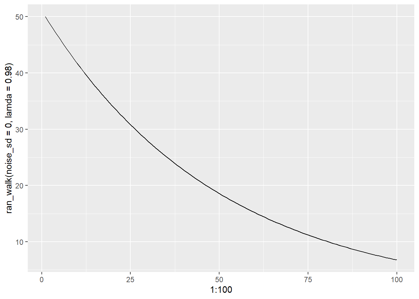
if lamda = 1.0, there will be no change in time step if lamda = 1.1, there will be a 10% increase each time step if lamda = 0.98, there will be a 2% decrease each time step
if lamda is > 1, we have a living organism
with stochastic, each time step can be up or down, but on average will be 0 due to normal distribution will keep track of what happens until we hit 0 in terms of real population, thats extinction <- this is where break comes into play ————————————————————————————
library(ggplot2)
ran_walk <- function(times=100,
                     n1=50,
                     lamda = 1.00,
                     noise_sd = 10) {
  n <- rep(NA, times) # create output vector
  n[1] <- n1 # initial population size
  noise <- rnorm(n = times, mean = 0, sd = noise_sd) # create noise vector
  # on average, noise should be 0 but some will be pos and some will be neg
  for(i in 1:(times-1)) {
    n[i+1] <- lamda*n[i] + noise[i]
   if(n[i + 1] <= 0) {
      n[i + 1] <- NA
      cat("Population extinction at time", i+1, "\n")
      break
    }
  }
  return(n)
}

# Testing ran_walk() function
# This function is an example of something that needs to be done in a for-loop
# do we want stop instead of break?
ran_walk()
## Population extinction at time 18## [1] 50.00000 55.02635 48.68178 42.52928 37.19796 30.70386 39.70569 24.27046
## [9] 27.13400 24.56143 29.31350 28.36519 34.61533 25.70124 23.62635 25.84784
## [17] 13.82831 NA NA NA NA NA NA NA
## [25] NA NA NA NA NA NA NA NA
## [33] NA NA NA NA NA NA NA NA
## [41] NA NA NA NA NA NA NA NA
## [49] NA NA NA NA NA NA NA NA
## [57] NA NA NA NA NA NA NA NA
## [65] NA NA NA NA NA NA NA NA
## [73] NA NA NA NA NA NA NA NA
## [81] NA NA NA NA NA NA NA NA
## [89] NA NA NA NA NA NA NA NA
## [97] NA NA NA NAUsing qplot with our new function <- but it was deprecated in 3.4.0 so be careful
## Warning: `qplot()` was deprecated in ggplot2 3.4.0.
## This warning is displayed once every 8 hours.
## Call `lifecycle::last_lifecycle_warnings()` to see where this warning was
## generated.
## Population extinction at time 25## Warning: Removed 76 rows containing missing values or values outside the scale range
## (`geom_line()`).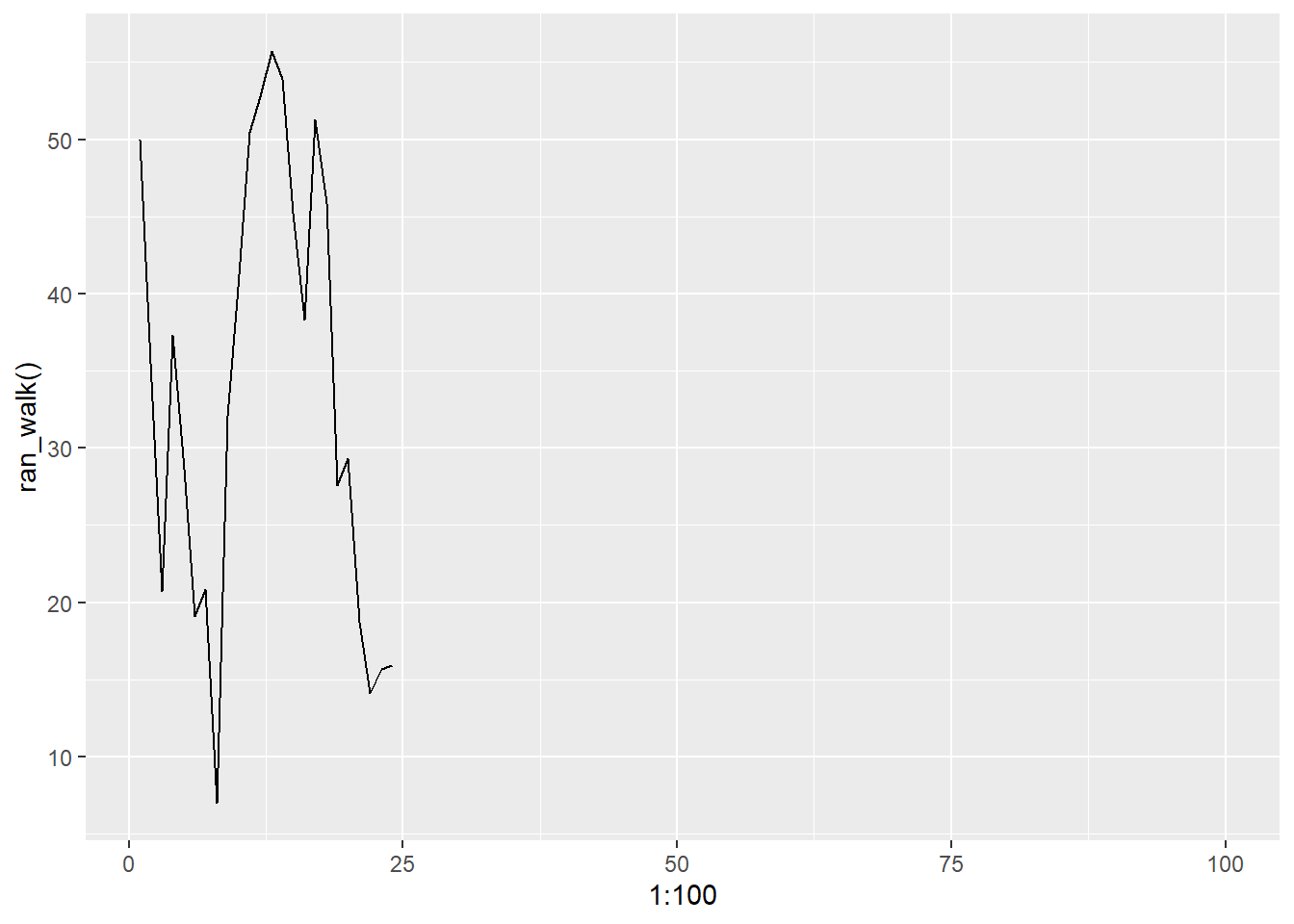
Now, time for test cases - o boy
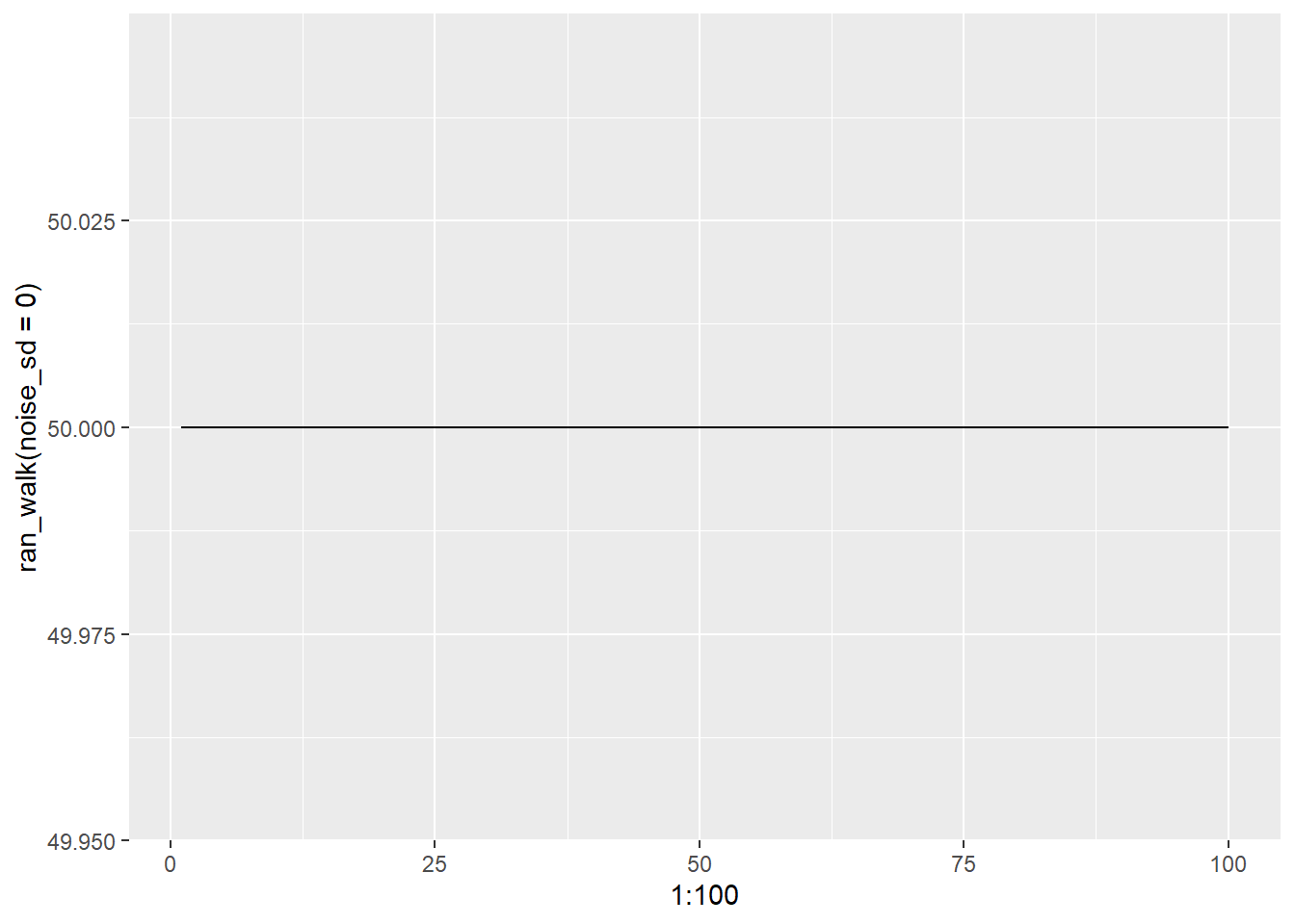
Checking our math, we see setting noise to 0 we get no change i.e. population stays stable
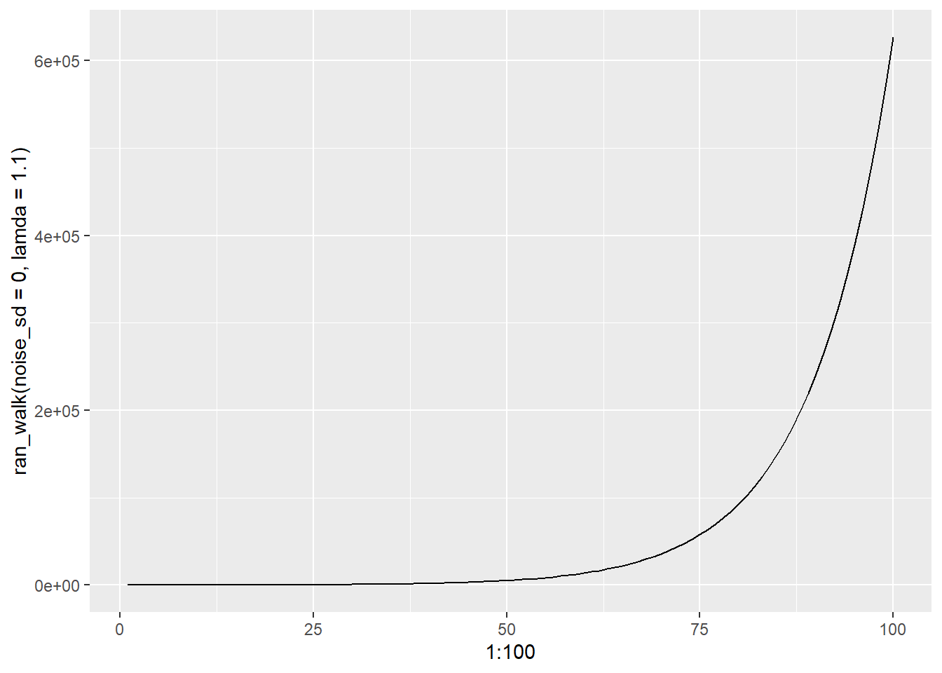
Now that we have seen exponential growth, lets see decay
Pure white noise
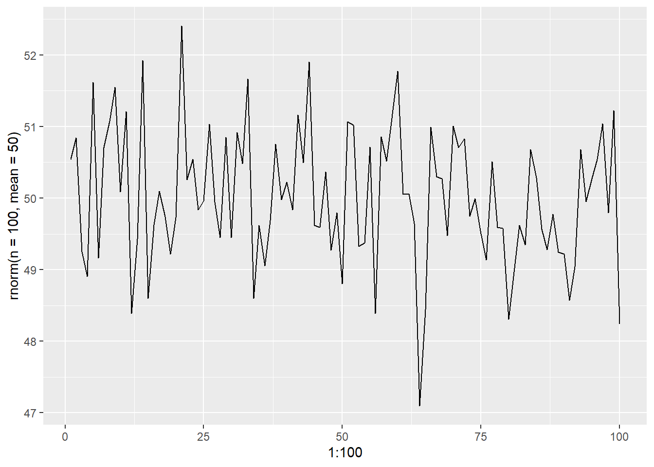
Could use round() function to keep integers
for sexual reproduction, what if all same sex? use unisexExtinct == runif(1) <= 2*(0.5)^n
environmental noise not random walk – add rnorm(0,1)
measurement error – add rnorm(0,1) for 0’s w/o extinction
Using double for loop - loop de loop
for test matrices, want them modularly sized and avoid square matrices if possible
looping over rows
##      [,1] [,2] [,3] [,4]
## [1,] 1.08 1.78 1.27 1.45
## [2,] 1.75 1.48 1.88 1.33
## [3,] 1.07 1.83 1.48 1.44
## [4,] 1.96 1.43 1.28 1.09
## [5,] 1.40 1.28 1.77 1.46
now looping over columns <- switched i with j, this will help with syntax and code reading
##      [,1] [,2] [,3] [,4]
## [1,] 2.08 2.78 2.27 2.45
## [2,] 2.75 2.48 2.88 2.33
## [3,] 2.07 2.83 2.48 2.44
## [4,] 2.96 2.43 2.28 2.09
## [5,] 2.40 2.28 2.77 2.46
Now building a double for-loop, or nested for-loop
m <- matrix(round(runif(20), digits = 2), nrow =5)
for (i in 1:nrow(m)) {
  for (k in 1:ncol(m)) {
    m[i,j] <- m[i,j] + i + j # taking number and adding values to it

  } # end of j loop
} # end of i loop
print(m)
## [,1] [,2] [,3] [,4]
## [1,] 0.37 0.61 0.14 20.27
## [2,] 0.40 0.82 0.41 24.34
## [3,] 0.31 0.35 0.20 28.77
## [4,] 0.22 0.88 0.40 32.40
## [5,] 0.15 0.59 0.12 36.57Creating function to sweep over parameters, including good formatting for function in code/comments <- from ecology
# Function: Species area curve <- S = cA^z
# Creates power function relationship for S and A
# input:  A is a vector of island areas
#         c is the intercept constant
#         z is the slope constant
# output: S is a vector of species richness values
#
#
# ----------------------------------------------------------

species_area_curve <- function(A=1:5000, c = 0.5, z = 0.26) {
  S <- c*(A^z)
  return(S)
}Creating Second function for plotting
# function: species_area_plot
# plot species area curves with parameter values
# input: A = vector of areas
#        c = single value for c parameter
#        z = single value for z paremeter
#
# output: smoothed curve with parameters in graph
# -----------------------------------------------
# Also examples of using functions within functions

species_area_plot <- function(A=1:5000, c = 0.5, z = 0.26) {
  plot(x = A, species_area_curve(A,c,z),
       type = "l",
       xlab = "Island Area",
       ylab = "S",
       ylim=c(0,2500))
  mtext(paste("c =", c, "z = ", z), cex = 0.7) # This code will put z and c values on top of graphs when called
  # return()

}
species_area_plot()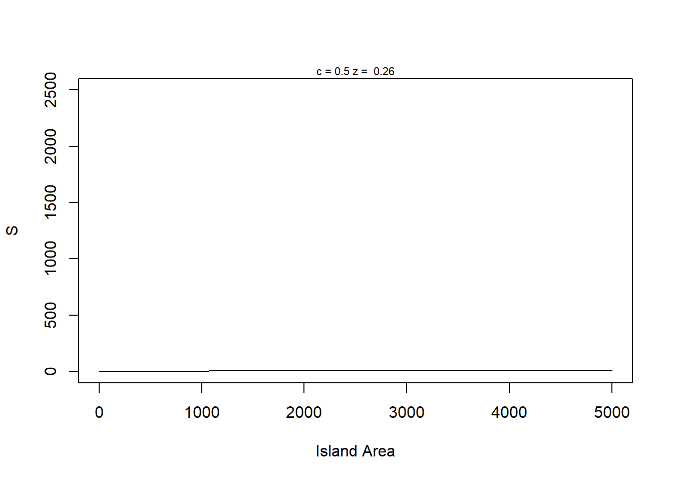
Declaring global vairables <- often called at beginning of code
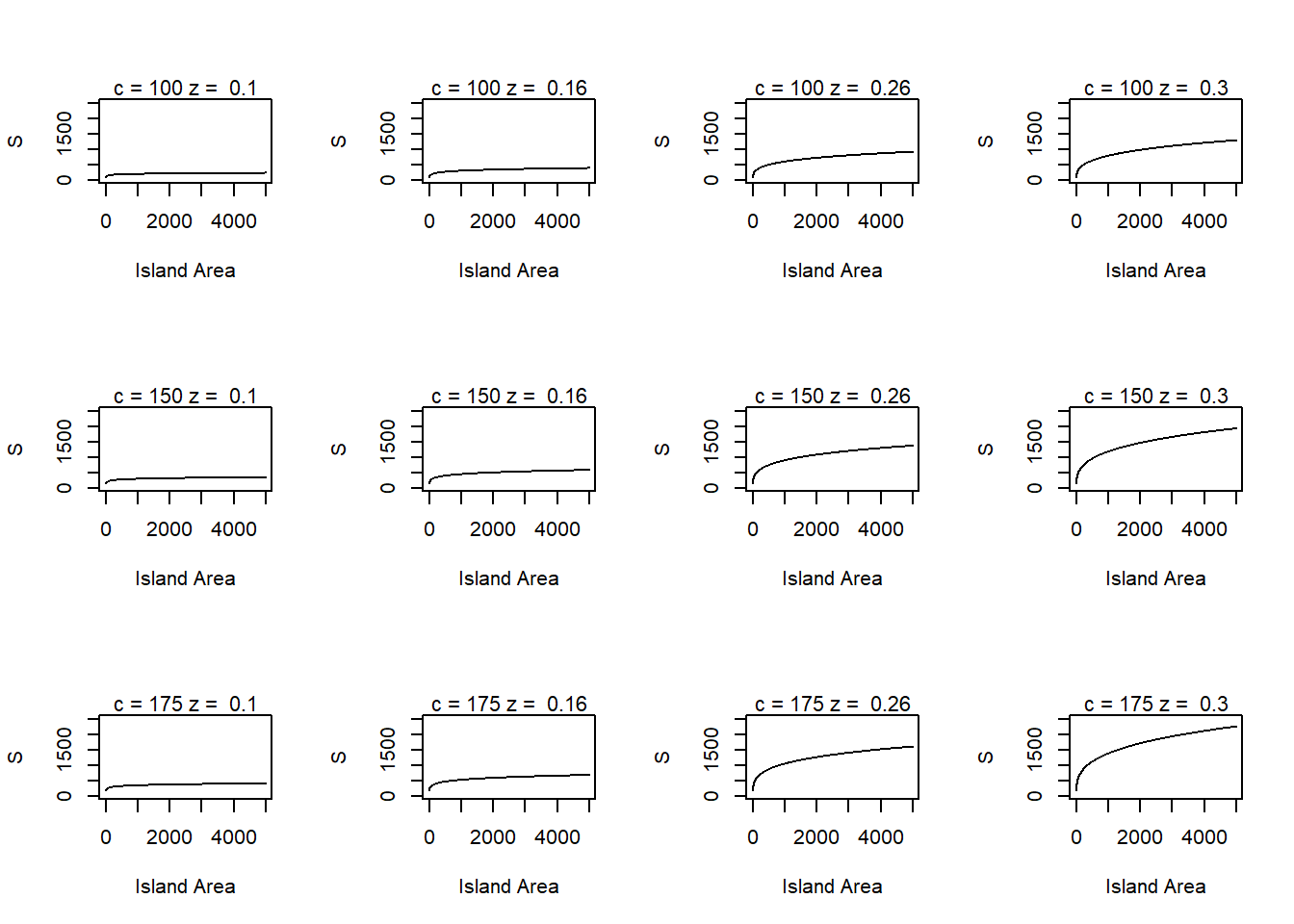
mfrow example
par(mfrow=c(3,4)) # mfrow calls to graphics display, unique to base R graphics
# This will be in a matrix structure and uses our previous function
for (i in seq_along(c_pars)) { # will jump over c_pars values
  for (j in seq_along(z_pars)) { # will jump over z_pars values
    species_area_plot(c=c_pars[i], z=z_pars[j]) # should in total make 12 passes through this and get a grid of 12 plots
  }
}
Comparing For and While loops
looping with for
This is a good example of calculating something of unspecified length
Similar to other languages, we will do a while loop
looping with while
NOTE:
if z = NA OR z is greater than or equal to cut_point, which is 0.1 loop will continue to run loop will stop when z is less than the cut_point or is NA instead of printing out loop number, since we do not have one, we print out cycle_number Though, while loops are generally bad practice - for loops are generally better form Worst part of while loop - unsure if it will ever end - I.E. it could never meet criteria then go on forever - no good for example, if cut_point is something so low like 0.00001, it could run for a while, no pun intended
## [1] 0.08370573## [1] 29Now using the repeat function
Expand grid function <- Mucho importante
This function automatically sets up variables and pairs up unique combination of the two inputted values c_pars is 3, z_pars is 4, so it gives us a data frame of 12 unique combinations using c_pars and z_pars from earlier, lines 206 and 207
##    Var1 Var2
## 1   100 0.10
## 2   150 0.10
## 3   175 0.10
## 4   100 0.16
## 5   150 0.16
## 6   175 0.16
## 7   100 0.26
## 8   150 0.26
## 9   175 0.26
## 10  100 0.30
## 11  150 0.30
## 12  175 0.30
expand.grid examples for creating data sets
df <- expand.grid(x = c_pars, y = z_pars) # x can be replaced with column/variable name for first value, y can be replaced for second value and so on
# can be down with more than 2 values
df2 <- expand.grid(x = c_pars, y = z_pars, z = c_pars*2) # now 36 values, 3*4*3 = 36
df2
## x y z
## 1 100 0.10 200
## 2 150 0.10 200
## 3 175 0.10 200
## 4 100 0.16 200
## 5 150 0.16 200
## 6 175 0.16 200
## 7 100 0.26 200
## 8 150 0.26 200
## 9 175 0.26 200
## 10 100 0.30 200
## 11 150 0.30 200
## 12 175 0.30 200
## 13 100 0.10 300
## 14 150 0.10 300
## 15 175 0.10 300
## 16 100 0.16 300
## 17 150 0.16 300
## 18 175 0.16 300
## 19 100 0.26 300
## 20 150 0.26 300
## 21 175 0.26 300
## 22 100 0.30 300
## 23 150 0.30 300
## 24 175 0.30 300
## 25 100 0.10 350
## 26 150 0.10 350
## 27 175 0.10 350
## 28 100 0.16 350
## 29 150 0.16 350
## 30 175 0.16 350
## 31 100 0.26 350
## 32 150 0.26 350
## 33 175 0.26 350
## 34 100 0.30 350
## 35 150 0.30 350
## 36 175 0.30 350## x y
## 1 100 0.10
## 2 150 0.10
## 3 175 0.10
## 4 100 0.16
## 5 150 0.16
## 6 175 0.16## 'data.frame': 12 obs. of 2 variables:
## $ x: num 100 150 175 100 150 175 100 150 175 100 ...
## $ y: num 0.1 0.1 0.1 0.16 0.16 0.16 0.26 0.26 0.26 0.3 ...
## - attr(*, "out.attrs")=List of 2
## ..$ dim : Named int [1:2] 3 4
## .. ..- attr(*, "names")= chr [1:2] "x" "y"
## ..$ dimnames:List of 2
## .. ..$ x: chr [1:3] "x=100" "x=150" "x=175"
## .. ..$ y: chr [1:4] "y=0.10" "y=0.16" "y=0.26" "y=0.30"## x y
## 1 100 0.10
## 2 150 0.10
## 3 175 0.10
## 4 100 0.16
## 5 150 0.16
## 6 175 0.16
## 7 100 0.26
## 8 150 0.26
## 9 175 0.26
## 10 100 0.30
## 11 150 0.30
## 12 175 0.30Creating sa_output function
This function gives us a 2 value list with x = max - min, and y = coefficient of variation
##################################################
# function: sa_output
# Summary stats for species-area power function
# input: vector of predicted species richness (right now random numeric value)
# output: list of max-min called sum_stats, coefficient of variation
#-------------------------------------------------

sa_output <- function(S=runif(10)) {

  sum_stats <- list(s_gain=max(S)-min(S),s_cv=sd(S)/mean(S)) # list of  first: max value of s - min of s,
  # then taking the standard deviation of s divided by the mean of s for second list value

  return(sum_stats)
}
sa_output() # list is 2 values
## $s_gain
## [1] 0.6699767
##
## $s_cv
## [1] 0.4095386Build program body with a single loop through the parameters in modelFrame
Global variables, area vector, c_pars again, and z_pars
set up model/data frame using expand.grid
model_frame <- expand.grid(c=c_pars,z=z_pars)
model_frame$s_gain <- NA # adding column called s_gain with values NA
model_frame$s_cv <- NA # adding column called s_cv with values NA
print(model_frame)
## c z s_gain s_cv
## 1 100 0.10 NA NA
## 2 150 0.10 NA NA
## 3 175 0.10 NA NA
## 4 100 0.16 NA NA
## 5 150 0.16 NA NA
## 6 175 0.16 NA NA
## 7 100 0.26 NA NA
## 8 150 0.26 NA NA
## 9 175 0.26 NA NA
## 10 100 0.30 NA NA
## 11 150 0.30 NA NA
## 12 175 0.30 NA NAcycle through model calculations - using multiple functions
starting from 1 to number of rows from model_frame - in our case, 12 rows
Replacing the values of NA from model_frame with our calculated values from our created functions
Notice, by using our functions and expand.grid we made this one_dimensional looping keeps values associated with appropriate rows
for (i in 1:nrow(model_frame)) {

  # generate S vector
  # calling upon species_area_curve from earlier and creating a temp value
  # Using area vector from earlier which is 1 to 5000
  # model_frame[i,1] will take row i, col 1, which is our c_par, c
  # model_frame[i,2] will take row i, col 2, which is our z_par, z
  temp1 <- species_area_curve(A=area,
                              c=model_frame[i,1],
                              z=model_frame[i,2])
  # calculate output stats using our first temp value, creating a second temp value
  # temp2 <- sa_output(temp1) < could use temp2 but uneccessary
  # model_frame[i,c(3,4)] <- temp2
  # temp 2 is a list, and then were passing this list into a model_frame which we need   # to do since were passing in multiple columns into a data frame
  # pass results to columns in data frame
  model_frame[i,c(3,4)] <- sa_output(temp1)

}
print(model_frame)
## c z s_gain s_cv
## 1 100 0.10 134.3673 0.09109192
## 2 150 0.10 201.5509 0.09109192
## 3 175 0.10 235.1428 0.09109192
## 4 100 0.16 290.6926 0.13905495
## 5 150 0.16 436.0389 0.13905495
## 6 175 0.16 508.7121 0.13905495
## 7 100 0.26 815.6557 0.21070232
## 8 150 0.26 1223.4835 0.21070232
## 9 175 0.26 1427.3975 0.21070232
## 10 100 0.30 1187.3333 0.23699746
## 11 150 0.30 1780.9999 0.23699746
## 12 175 0.30 2077.8333 0.23699746Parameter Sweeping Redux using ggplot to graph the data
First, global variables for loops for data
set up model frame, this time with col S that has values NA and we have col A
model_frame will be 5 * 3 * 4 = 60 rows/combinations large
##      c    z A  S
## 1  100 0.10 1 NA
## 2  150 0.10 1 NA
## 3  175 0.10 1 NA
## 4  100 0.16 1 NA
## 5  150 0.16 1 NA
## 6  175 0.16 1 NA
## 7  100 0.26 1 NA
## 8  150 0.26 1 NA
## 9  175 0.26 1 NA
## 10 100 0.30 1 NA
## 11 150 0.30 1 NA
## 12 175 0.30 1 NA
## 13 100 0.10 2 NA
## 14 150 0.10 2 NA
## 15 175 0.10 2 NA
## 16 100 0.16 2 NA
## 17 150 0.16 2 NA
## 18 175 0.16 2 NA
## 19 100 0.26 2 NA
## 20 150 0.26 2 NA
## 21 175 0.26 2 NA
## 22 100 0.30 2 NA
## 23 150 0.30 2 NA
## 24 175 0.30 2 NA
## 25 100 0.10 3 NA
## 26 150 0.10 3 NA
## 27 175 0.10 3 NA
## 28 100 0.16 3 NA
## 29 150 0.16 3 NA
## 30 175 0.16 3 NA
## 31 100 0.26 3 NA
## 32 150 0.26 3 NA
## 33 175 0.26 3 NA
## 34 100 0.30 3 NA
## 35 150 0.30 3 NA
## 36 175 0.30 3 NA
## 37 100 0.10 4 NA
## 38 150 0.10 4 NA
## 39 175 0.10 4 NA
## 40 100 0.16 4 NA
## 41 150 0.16 4 NA
## 42 175 0.16 4 NA
## 43 100 0.26 4 NA
## 44 150 0.26 4 NA
## 45 175 0.26 4 NA
## 46 100 0.30 4 NA
## 47 150 0.30 4 NA
## 48 175 0.30 4 NA
## 49 100 0.10 5 NA
## 50 150 0.10 5 NA
## 51 175 0.10 5 NA
## 52 100 0.16 5 NA
## 53 150 0.16 5 NA
## 54 175 0.16 5 NA
## 55 100 0.26 5 NA
## 56 150 0.26 5 NA
## 57 175 0.26 5 NA
## 58 100 0.30 5 NA
## 59 150 0.30 5 NA
## 60 175 0.30 5 NA
2 dimensional for loop through the parameters and fill column S with SA function values
for (i in 1:length(c_pars)) {
  for (j in 1:length(z_pars)) {
    model_frame[model_frame$c==c_pars[i] & model_frame$z==z_pars[j],"S"] <-   species_area_curve(A=area,c=c_pars[i],z=z_pars[j])
  }
}
model_frame
## c z A S
## 1 100 0.10 1 100.0000
## 2 150 0.10 1 150.0000
## 3 175 0.10 1 175.0000
## 4 100 0.16 1 100.0000
## 5 150 0.16 1 150.0000
## 6 175 0.16 1 175.0000
## 7 100 0.26 1 100.0000
## 8 150 0.26 1 150.0000
## 9 175 0.26 1 175.0000
## 10 100 0.30 1 100.0000
## 11 150 0.30 1 150.0000
## 12 175 0.30 1 175.0000
## 13 100 0.10 2 107.1773
## 14 150 0.10 2 160.7660
## 15 175 0.10 2 187.5604
## 16 100 0.16 2 111.7287
## 17 150 0.16 2 167.5931
## 18 175 0.16 2 195.5252
## 19 100 0.26 2 119.7479
## 20 150 0.26 2 179.6218
## 21 175 0.26 2 209.5588
## 22 100 0.30 2 123.1144
## 23 150 0.30 2 184.6717
## 24 175 0.30 2 215.4503
## 25 100 0.10 3 111.6123
## 26 150 0.10 3 167.4185
## 27 175 0.10 3 195.3216
## 28 100 0.16 3 119.2173
## 29 150 0.16 3 178.8260
## 30 175 0.16 3 208.6303
## 31 100 0.26 3 133.0612
## 32 150 0.26 3 199.5918
## 33 175 0.26 3 232.8571
## 34 100 0.30 3 139.0389
## 35 150 0.30 3 208.5584
## 36 175 0.30 3 243.3181
## 37 100 0.10 4 114.8698
## 38 150 0.10 4 172.3048
## 39 175 0.10 4 201.0222
## 40 100 0.16 4 124.8331
## 41 150 0.16 4 187.2496
## 42 175 0.16 4 218.4578
## 43 100 0.26 4 143.3955
## 44 150 0.26 4 215.0933
## 45 175 0.26 4 250.9422
## 46 100 0.30 4 151.5717
## 47 150 0.30 4 227.3575
## 48 175 0.30 4 265.2504
## 49 100 0.10 5 117.4619
## 50 150 0.10 5 176.1928
## 51 175 0.10 5 205.5583
## 52 100 0.16 5 129.3705
## 53 150 0.16 5 194.0557
## 54 175 0.16 5 226.3983
## 55 100 0.26 5 151.9610
## 56 150 0.26 5 227.9415
## 57 175 0.26 5 265.9318
## 58 100 0.30 5 162.0657
## 59 150 0.30 5 243.0985
## 60 175 0.30 5 283.61491 dimensional for loop that assigns values of species_area_curve function to col S of model_frame, where the parameters for the function are the corresponding rows should be same values
Real power of expand.grid <- goes through 3 columns for 1 row in one call
Does not have to loop over parameters
for (i in 1:nrow(model_frame)) {
  model_frame[i,"S"] <- species_area_curve(A=model_frame$A[i],
                                           c=model_frame$c[i],
                                           z=model_frame$z[i])
}
print(model_frame) # check by printing a data frame with limited parameter values
## c z A S
## 1 100 0.10 1 100.0000
## 2 150 0.10 1 150.0000
## 3 175 0.10 1 175.0000
## 4 100 0.16 1 100.0000
## 5 150 0.16 1 150.0000
## 6 175 0.16 1 175.0000
## 7 100 0.26 1 100.0000
## 8 150 0.26 1 150.0000
## 9 175 0.26 1 175.0000
## 10 100 0.30 1 100.0000
## 11 150 0.30 1 150.0000
## 12 175 0.30 1 175.0000
## 13 100 0.10 2 107.1773
## 14 150 0.10 2 160.7660
## 15 175 0.10 2 187.5604
## 16 100 0.16 2 111.7287
## 17 150 0.16 2 167.5931
## 18 175 0.16 2 195.5252
## 19 100 0.26 2 119.7479
## 20 150 0.26 2 179.6218
## 21 175 0.26 2 209.5588
## 22 100 0.30 2 123.1144
## 23 150 0.30 2 184.6717
## 24 175 0.30 2 215.4503
## 25 100 0.10 3 111.6123
## 26 150 0.10 3 167.4185
## 27 175 0.10 3 195.3216
## 28 100 0.16 3 119.2173
## 29 150 0.16 3 178.8260
## 30 175 0.16 3 208.6303
## 31 100 0.26 3 133.0612
## 32 150 0.26 3 199.5918
## 33 175 0.26 3 232.8571
## 34 100 0.30 3 139.0389
## 35 150 0.30 3 208.5584
## 36 175 0.30 3 243.3181
## 37 100 0.10 4 114.8698
## 38 150 0.10 4 172.3048
## 39 175 0.10 4 201.0222
## 40 100 0.16 4 124.8331
## 41 150 0.16 4 187.2496
## 42 175 0.16 4 218.4578
## 43 100 0.26 4 143.3955
## 44 150 0.26 4 215.0933
## 45 175 0.26 4 250.9422
## 46 100 0.30 4 151.5717
## 47 150 0.30 4 227.3575
## 48 175 0.30 4 265.2504
## 49 100 0.10 5 117.4619
## 50 150 0.10 5 176.1928
## 51 175 0.10 5 205.5583
## 52 100 0.16 5 129.3705
## 53 150 0.16 5 194.0557
## 54 175 0.16 5 226.3983
## 55 100 0.26 5 151.9610
## 56 150 0.26 5 227.9415
## 57 175 0.26 5 265.9318
## 58 100 0.30 5 162.0657
## 59 150 0.30 5 243.0985
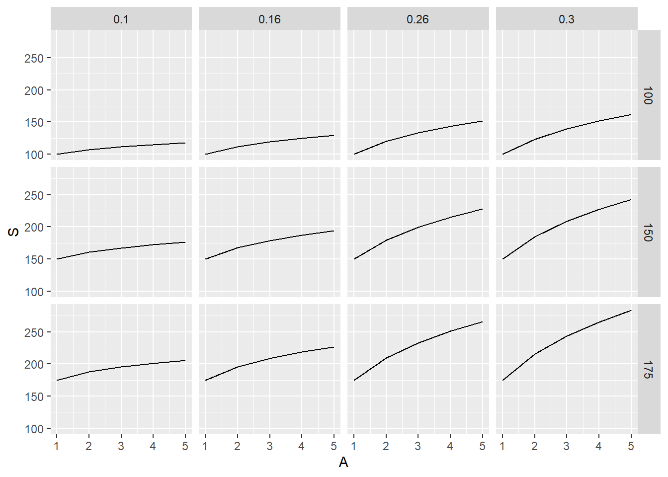
## 60 175 0.30 5 283.6149Now graphing this with ggplot, first - call upon ggplot2 - notice we dont need for-loops for this <- Abusing R’s vectorization
assigning plot of data of model_frame to p1 then adding comparison/graph details using geom_line
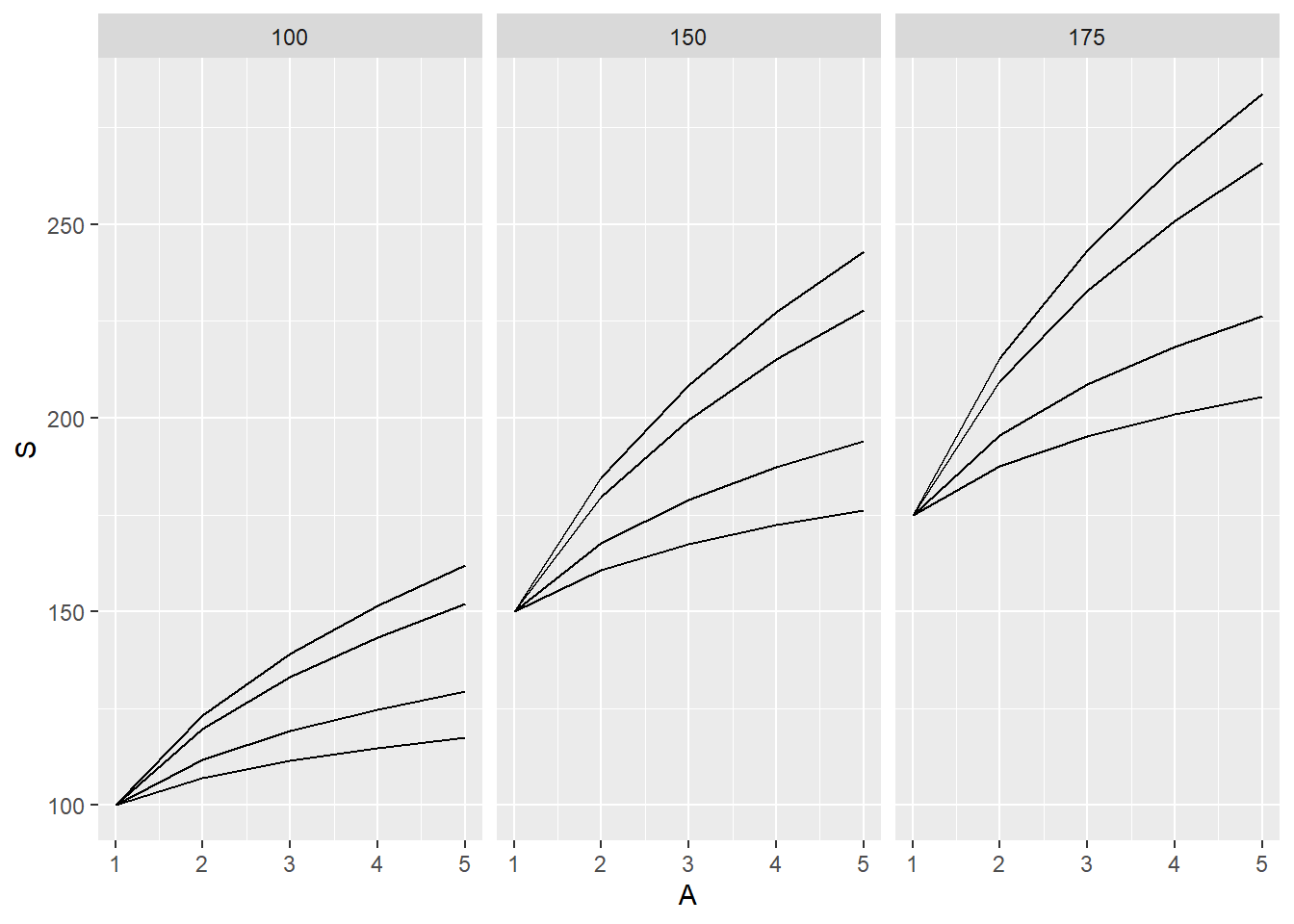
returns 12 graphs in one image
geom_line <- geometric/image ggplot will make, in this case a line with:
x axis is area (1,2,3,4,5), y value/axis is s (what we calculated)
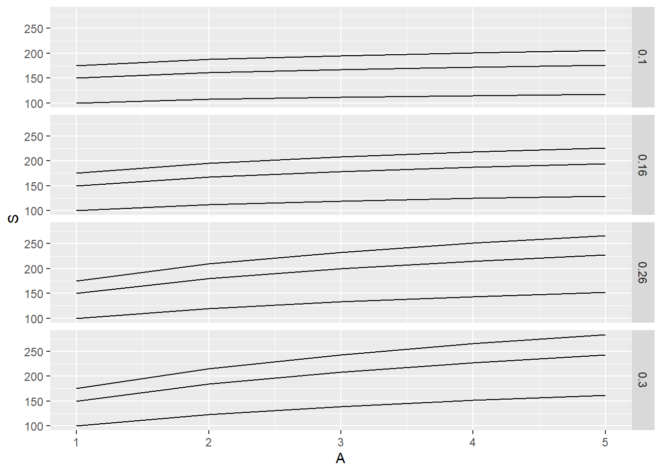
using facet_grid, our graphs are set up to show graphs for each c and z combination
Therefore, 12 graphs
don’t need $ for referencing data.col names as we specified data in our p1 variable
returns 3 graphs, each graph has 4 lines (values from z) for each c, giving us 3 graphs
Grouped by c values
notice the change in facet_grid, now it is saying all z values for each c